Speed Up Your Code: Parallel Processing with multidplyr
Written
There’s nothing more frustrating than waiting for long-running R scripts to iteratively run. I’ve recently come across a new-ish package for parallel processing that plays nicely with the tidyverse: multidplyr. The package has saved me countless hours when applied to long-running, iterative scripts. In this post, I’ll discuss the workflow to parallelize your code, and I’ll go through a real world example of collecting stock prices where it improves speed by over 5X for a process that normally takes 2 minutes or so. Once you grasp the workflow, the parallelization can be applied to almost any iterative scripts regardless of application.
Table of Contents
Prerequisites
The multidplyr package is not available on CRAN, but you can install it using devtools:
install.packages("devtools")
devtools::install_github("hadley/multidplyr")
For those following along in R, you’ll need to load the following packages, which are available on CRAN:
library(multidplyr) # parallel processing
library(rvest)      # web scraping
library(quantmod)   # get stock prices; useful stock analysis functions
library(tidyverse)  # ggplot2, purrr, dplyr, tidyr, readr, tibble
library(stringr)    # working with strings
library(lubridate)  # working with dates
If you don’t have these installed, run install.packages(pkg_names) with the package names as a character vector (pkg_names <- c("rvest", "quantmod", ...)).
I also recommend the open-source RStudio IDE, which makes R Programming easy and efficient.
Why Parallel Processing?
Computer programming languages, including R and python, by default run scripts using only one processor (i.e. core). Under many circumstances this is fine since the computation speed is relatively fast. However, some scripts just take a long time to process, particularly during iterative programming (i.e. using loops to process a lot of data and/or very complex calculations).
Most modern PC’s have multiple cores that are underutilized. Parallel processing takes advantage of this by splitting the work across the multiple cores for maximum processor utilization. The result is a dramatic improvement in processing time.
While you may not realize it, most computations in R are loops that can be split using parallel processing. However, parallel processing takes more code and may not improve speeds, especially during fast computations because it takes time to transmit and recombine data. Therefore, parallel processing should only be used when speed is a significant issue.
When processing time is long, parallel processing could result in a significant improvement. Let’s check out how to parallelie your R code using the multidplyr package.
Workflow
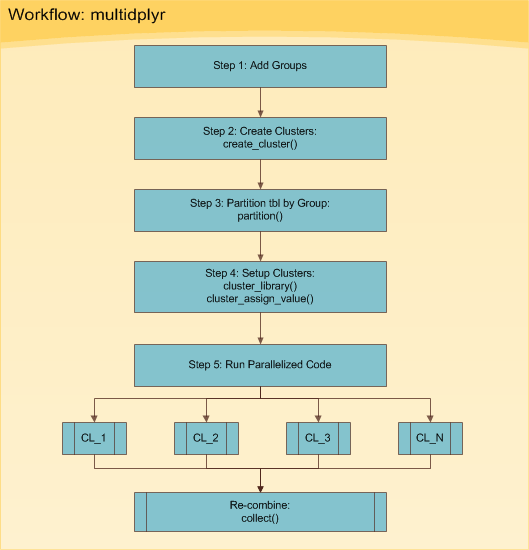
The multidplyr workflow can be broken down into six basic steps shown in Figure 1. The six steps are implemented in Processing in Parallel.
Figure 1: multidplyr Workflow
Essentially, you start with some data set that you need to do things to multiple times. Your situation generally falls into one of two types:
- It could be a really large data set that you want to split up into several small data sets and perform the same thing on each.
- It could be one data set that you want to perform multiple things on (e.g. apply many models).
The good news is both situations follow the same basic workflow. The toughest part is getting your data in the format needed to process using the workflow. Don’t worry, we’ll go through a real world example next so you can see how this is accomplished.
Real World Example
We’ll go through the multidplyr workflow using a real world example that I routinely use: collecting stock prices from the inter-web. Other uses include using modeling functions over grouped data sets, using many models on the same data set, and processing text (e.g. getting n-grams on large corpora). Basically anything with a loop.
Prep-Work
In preparation for collecting stock prices, we need two things:
- A list of stocks
- A function to get stock prices from a stock symbol
The code below comes from my S&P500 Stock Analysis Post and it is also used in my more advanced Russell 2000 Analysis Post.
First, we use rvest to get the list of S&P500 stocks, sp500.
library(rvest)
# Web-scrape SP500 stock list from Wikipedia
sp_500 <- read_html("https://en.wikipedia.org/wiki/List_of_S%26P_500_companies") %>%
    html_node("table.wikitable") %>%
    html_table() %>%
    select(`Ticker symbol`, Security) %>%
    as_tibble() %>%
    rename(symbol = `Ticker symbol`,
           company = Security)
# Show results
sp_500
## # A tibble: 505 × 2
##    symbol             company
##     <chr>               <chr>
## 1     MMM          3M Company
## 2     ABT Abbott Laboratories
## 3    ABBV              AbbVie
## 4     ACN       Accenture plc
## 5    ATVI Activision Blizzard
## 6     AYI   Acuity Brands Inc
## 7    ADBE   Adobe Systems Inc
## 8     AAP  Advance Auto Parts
## 9     AES            AES Corp
## 10    AET           Aetna Inc
## # ... with 495 more rows
Second, we create a function that leverages the quantmod::getSymbols to return the historical stock prices in tidy format. This function will be mapped to all of the 500+ stocks next.
library(quantmod)
# Function to Get Stock Prices in Tidy Form
get_stock_prices <- function(symbol, return_format = "tibble", ...) {
    # Get stock prices; Handle errors
    stock_prices <- tryCatch({
        getSymbols(Symbols = symbol, auto.assign = FALSE, ...)
    }, error = function(e) {
        return(NA) # Return NA on error
    })
    if (!is.na(stock_prices[[1]])) {
        # Rename
        names(stock_prices) <- c("Open", "High", "Low", "Close", "Volume", "Adjusted")
        # Return in xts format if tibble is not specified
        if (return_format == "tibble") {
            stock_prices <- stock_prices %>%
                as_tibble() %>%
                rownames_to_column(var = "Date") %>%
                mutate(Date = ymd(Date))
        }
        return(stock_prices)
    }
}
Processing In Series
The next computation is the routine that we wish to parallelize, but first we’ll time the script running on one processor, looping in series. We are collecting ten years of historical daily stock prices for each of the 500+ stocks. To do this, the script below uses the purrr::map() function to map get_stock_prices() to each stock symbol in sp_500. The loop in our case is the iterative application of a function to each stock. This operation will be split by group in the next section. The proc.time() function is used to time the routine running without parallel processing.
# Map get_stock_prices() to list of stock symbols
from <- "2007-01-01"
to   <- today()

start <- proc.time() # Start clock
sp_500_processed_in_series <- sp_500 %>%
    mutate(
        stock.prices = map(.x = symbol,
                           ~ get_stock_prices(symbol = .x,
                                              return_format = "tibble",
                                              from = from,
                                              to   = to)
                           )
        )
time_elapsed_series <- proc.time() - start # End clock
The result, sp_500_processed_in_series is a tibble (tidy data frame) that is nested with two levels: the first has the stock symbol, company, and stock.prices. The variable, stock.prices, contains the historical stock prices for each stock.
sp_500_processed_in_series
## # A tibble: 505 × 3
##    symbol             company         stock.prices
##     <chr>               <chr>               <list>
## 1     MMM          3M Company <tibble [2,506 × 7]>
## 2     ABT Abbott Laboratories <tibble [2,506 × 7]>
## 3    ABBV              AbbVie   <tibble [996 × 7]>
## 4     ACN       Accenture plc <tibble [2,506 × 7]>
## 5    ATVI Activision Blizzard <tibble [2,506 × 7]>
## 6     AYI   Acuity Brands Inc <tibble [2,506 × 7]>
## 7    ADBE   Adobe Systems Inc <tibble [2,506 × 7]>
## 8     AAP  Advance Auto Parts <tibble [2,506 × 7]>
## 9     AES            AES Corp <tibble [2,506 × 7]>
## 10    AET           Aetna Inc <tibble [2,506 × 7]>
## # ... with 495 more rows
Let’s verify we got the daily stock prices for every stock. We’ll use the tidyr::unnest() function to expand the stock.prices for the list of stocks. At 1,203,551 rows, the full list has been obtained.
sp_500_processed_in_series %>% unnest()
## # A tibble: 1,203,551 × 9
##    symbol    company       Date  Open  High   Low Close  Volume
##     <chr>      <chr>     <date> <dbl> <dbl> <dbl> <dbl>   <dbl>
## 1     MMM 3M Company 2007-01-03 77.53 78.85 77.38 78.26 3781500
## 2     MMM 3M Company 2007-01-04 78.40 78.41 77.45 77.95 2968400
## 3     MMM 3M Company 2007-01-05 77.89 77.90 77.01 77.42 2765200
## 4     MMM 3M Company 2007-01-08 77.42 78.04 76.97 77.59 2434500
## 5     MMM 3M Company 2007-01-09 78.00 78.23 77.44 77.68 1896800
## 6     MMM 3M Company 2007-01-10 77.31 77.96 77.04 77.85 1787500
## 7     MMM 3M Company 2007-01-11 78.05 79.03 77.88 78.65 2372500
## 8     MMM 3M Company 2007-01-12 78.41 79.50 78.22 79.36 2582200
## 9     MMM 3M Company 2007-01-16 79.48 79.62 78.92 79.56 2526600
## 10    MMM 3M Company 2007-01-17 79.33 79.51 78.75 78.91 2711300
## # ... with 1,203,541 more rows, and 1 more variables: Adjusted <dbl>
And, let’s see how long it took when processing in series. The processing time is the time elapsed in seconds. Converted to minutes this is approximately 1.68 minutes.
time_elapsed_series
##    user  system elapsed
##   43.12    1.08  100.58
Processing in Parallel
We just collected ten years of daily stock prices for over 500 stocks in about 1.68 minutes. Let’s parallelize the computation to get an improvement. We will follow the six steps shown in Figure 1.
Step 0: Get Number of Cores (Optional)
Prior to starting, you may want to determine how many cores your machine has. An easy way to do this is using parallel::detectCores(). This will be used to determine the number of groups to split the data into in the next set.
library(parallel)
cl <- detectCores()
cl
## [1] 8
Step 1: Add Groups
Let’s add groups to sp_500. The groups are needed to divide the data across your cl number cores. For me, this is 8 cores. We create a group vector, which is a sequential vector of 1:cl (1 to 8) repeated the length of the number of rows in sp_500. We then add the group vector to the sp_500 tibble using the dplyr::bind_cols() function.
group <- rep(1:cl, length.out = nrow(sp_500))
sp_500 <- bind_cols(tibble(group), sp_500)
sp_500
## # A tibble: 505 × 3
##    group symbol             company
##    <int>  <chr>               <chr>
## 1      1    MMM          3M Company
## 2      2    ABT Abbott Laboratories
## 3      3   ABBV              AbbVie
## 4      4    ACN       Accenture plc
## 5      5   ATVI Activision Blizzard
## 6      6    AYI   Acuity Brands Inc
## 7      7   ADBE   Adobe Systems Inc
## 8      8    AAP  Advance Auto Parts
## 9      1    AES            AES Corp
## 10     2    AET           Aetna Inc
## # ... with 495 more rows
Step 2: Create Clusters
Use the create_cluster() function from the multidplyr package. Think of a cluster as a work environment on a core. Therefore, the code below establishes a work environment on each of the 8 cores.
cluster <- create_cluster(cores = cl)
cluster
## socket cluster with 8 nodes on host 'localhost'
Step 3: Partition by Group
Next is partitioning. Think of partitioning as sending a subset of the initial tibble to each of the clusters. The result is a partitioned data frame (party_df), which we explore next. Use the partition() function from the multidplyr package to split the sp_500 list by group and send each group to a different cluster.
by_group <- sp_500 %>%
    partition(group, cluster = cluster)
by_group
## Source: party_df [505 x 3]
## Groups: group
## Shards: 8 [63--64 rows]
##
## # S3: party_df
##    group symbol                           company
##    <int>  <chr>                             <chr>
## 1      6    AYI                 Acuity Brands Inc
## 2      6    APD      Air Products & Chemicals Inc
## 3      6    ADS             Alliance Data Systems
## 4      6    AEP           American Electric Power
## 5      6   AMGN                         Amgen Inc
## 6      6   AAPL                        Apple Inc.
## 7      6    ADP         Automatic Data Processing
## 8      6     BK The Bank of New York Mellon Corp.
## 9      6   BIIB                  BIOGEN IDEC Inc.
## 10     6   AVGO                          Broadcom
## # ... with 495 more rows
The result, by_group, looks similar to our original tibble, but it is a party_df, which is very different. The key is to notice that the there are 8 Shards. Each Shard has between 63 and 64 rows, which evenly splits our data among each shard. Now that our tibble has been partitioned into a party_df, we are ready to move onto setting up the clusters.
Step 4: Setup Clusters
The clusters have a local, bare-bones R work environment, which doesn’t work for the vast majority of cases. Code typically depends on libraries, functions, expressions, variables, and/or data that are not available in base R. Fortunately, there is a way to add these items to the clusters. Let’s see how.
For our computation, we are going to need to add several libraries along with the get_stock_prices() function to the clusters. We do this by using the cluster_library() and cluster_assign_value() functions, respectively.
from <- "2007-01-01"
to   <- today()
# Utilize pipe (%>%) to assign libraries, functions, and values to clusters
by_group %>%
    # Assign libraries
    cluster_library("tidyverse") %>%
    cluster_library("stringr") %>%
    cluster_library("lubridate") %>%
    cluster_library("quantmod") %>%
    # Assign values (use this to load functions or data to each core)
    cluster_assign_value("get_stock_prices", get_stock_prices) %>%
    cluster_assign_value("from", from) %>%
    cluster_assign_value("to", to)
We can verify that the libraries are loaded using the cluster_eval() function.
cluster_eval(by_group, search())[[1]] # results for first cluster shown only
##  [1] ".GlobalEnv"        "package:quantmod"  "package:TTR"
##  [4] "package:xts"       "package:zoo"       "package:lubridate"
##  [7] "package:stringr"   "package:dplyr"     "package:purrr"
## [10] "package:readr"     "package:tidyr"     "package:tibble"
## [13] "package:ggplot2"   "package:tidyverse" "package:stats"
## [16] "package:graphics"  "package:grDevices" "package:utils"
## [19] "package:datasets"  "package:methods"   "Autoloads"
## [22] "package:base"
We can also verify that the functions are loaded using the cluster_get() function.
cluster_get(by_group, "get_stock_prices")[[1]] # results for first cluster shown only
## function(symbol, return_format = "tibble", ...) {
##     # Get stock prices; Handle errors
##     stock_prices <- tryCatch({
##         getSymbols(Symbols = symbol, auto.assign = FALSE, ...)
##     }, error = function(e) {
##         return(NA) # Return NA on error
##     })
##     if (!is.na(stock_prices[[1]])) {
##         # Rename
##         names(stock_prices) <- c("Open", "High", "Low", "Close", "Volume", "Adjusted")
##         # Return in xts format if tibble is not specified
##         if (return_format == "tibble") {
##             stock_prices <- stock_prices %>%
##                 as_tibble() %>%
##                 rownames_to_column(var = "Date") %>%
##                 mutate(Date = ymd(Date))
##         }
##         return(stock_prices)
##     }
## }
Step 5: Run Parallelized Code
Now that we have our clusters and partitions set up and everything looks good, we can run the parallelized code. The code chunk is the same as the series code chunk with two exceptions:
- Instead of starting with the
sp_500 tibble, we start with the by_group party_df
- We combine the results at the end using the
collect() function
start <- proc.time() # Start clock
sp_500_processed_in_parallel <- by_group %>% # Use by_group party_df
    mutate(
        stock.prices = map(.x = symbol,
                           ~ get_stock_prices(symbol = .x,
                                              return_format = "tibble",
                                              from = from,
                                              to   = to)
                           )
        ) %>%
    collect() %>% # Special collect() function to recombine partitions
    as_tibble()   # Convert to tibble
time_elapsed_parallel <- proc.time() - start # End clock
Let’s verify we got the list of stock prices. We’ll use the tidyr::unnest() function to expand the stock.prices for the list of stocks. This is the same list as sp_500_processed_in_series, but it’s sorted in order by which groups finished first. If we want to return the tibble in the same order of sp_500, we can easily pipe (%>%) arrange(company) after as_tibble() in the code chunk above.
sp_500_processed_in_parallel %>% unnest()
## Source: local data frame [1,204,056 x 10]
## Groups: group [8]
##
##    group symbol           company       Date  Open  High   Low Close
##    <int>  <chr>             <chr>     <date> <dbl> <dbl> <dbl> <dbl>
## 1      6    AYI Acuity Brands Inc 2007-01-03 52.20 53.27 51.52 51.92
## 2      6    AYI Acuity Brands Inc 2007-01-04 53.00 53.39 49.69 52.32
## 3      6    AYI Acuity Brands Inc 2007-01-05 51.74 51.85 50.95 51.09
## 4      6    AYI Acuity Brands Inc 2007-01-08 51.15 52.64 50.70 52.01
## 5      6    AYI Acuity Brands Inc 2007-01-09 51.94 52.59 51.66 52.52
## 6      6    AYI Acuity Brands Inc 2007-01-10 52.13 53.61 52.01 53.48
## 7      6    AYI Acuity Brands Inc 2007-01-11 53.60 55.47 53.52 55.08
## 8      6    AYI Acuity Brands Inc 2007-01-12 54.84 55.68 54.61 55.65
## 9      6    AYI Acuity Brands Inc 2007-01-16 55.65 56.56 55.40 55.61
## 10     6    AYI Acuity Brands Inc 2007-01-17 55.56 56.32 55.20 55.90
## # ... with 1,204,046 more rows, and 2 more variables: Volume <dbl>,
## #   Adjusted <dbl>
And, let’s see how long it took when processing in parallel.
time_elapsed_parallel
##    user  system elapsed
##    0.17    0.28   18.66
The processing time is approximately 0.31 minutes, which is 5.4X faster! Note that it’s not a full 8X faster because of transmission time as data is sent to and from the nodes. With that said, the speed will approach 8X improvement as calculations become longer since the transmission time is fixed whereas the computation time is variable.
Conclusion
Parallelizing code can drastically improve speed on multi-core machines. It makes the most sense in situations involving many iterative computations. On an 8 core machine, processing time significantly improves. It will not be quite 8X faster, but the longer the computation the closer the speed gets to the full 8X improvement. For a computation that takes two minutes under normal conditions, we improved the processing speed by over 5X through parallel processing!
Recap
The focus of this post was on the multidplyr package, a package designed to do parallel processing within the tidyverse. We worked through the five main steps in the multidplyr workflow on a real world example of collecting historical stock prices for a large set of stocks. The beauty is that the package and workflow can be applied to anything from collecting stocks to applying many models to computing n-grams on textual data and more!
Further Reading
multidplyr on GitHub: The vignette explains the multidplyr workflow using the flights data set from the nycflights13 package.